Context
Being known to the general public is the key to success in the music industry. Nowadays, an artist is considered popular if they manage to break into the top charts of Spotify, a digital music, podcast, and video streaming platform. Being able to predict the popularity of a song can help an artist to improve their track and adapt it to trends before its release. For a label, it can guide their selection of which artists to sign or which track on an album to promote as a single. Popularity of songs will therefore be predicted based on statistics about the song’s audio (tempo, key, danceability) and data like artist name and track genre.
Dataset Analysed
The dataset used for this analysis is generated from the Spotify API and spans 176,774 songs. It contains 18 features with information about the song, two of them are non-predictive and one of them, popularity, is this report's goal field. Popularity is a value between 0 and 100 generated by Spotify, its computation is based on the total number of plays compared to other tracks as well as how recent those plays are.
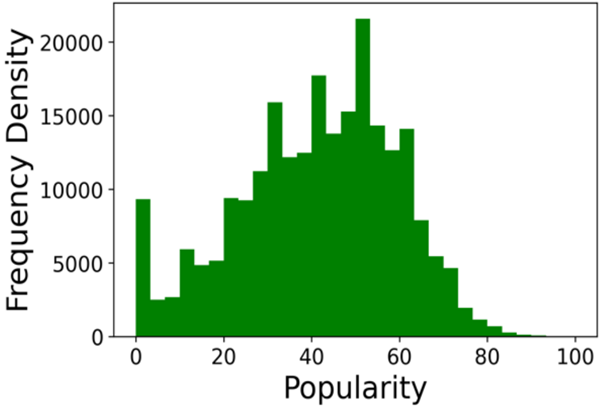 Figure 1. Frequency of Popularity values 0-100
Data preparation
Firstly, duplicate songs had to be dropped. Some tracks with the same individual track ID were listed multiple times with different genre values. By removing these, the dataset was reduced from 232,725 songs to 176,774. Secondly, the non-predictive attributes were removed. These included the track ID, which is just a tag attached to the song so it can be identified and the track name, which, because of its high cardinality, made pre-processing very complex. Extracting key words from the track name was considered as they could have high predictive values, but this was not carried out. The data then only contained predictive values and the goal field which were separated in x and y values, with y being the ‘popularity’ and x being the other features. The data was split, 80% for training and 20% for testing and validation. Repeated k-fold cross validation was used so the testing and validation did not need to be allocated separately. The attributes were sorted into numerical and categorical groups to be processed differently. The categorical group was then split again to separate artist_name. Through using a pipeline and a column transformer the pre-processing steps could be chained and the groups of attributes could be treated differently:
- The numerical data was cleaned and then scaled so the attributes were inter-comparable. This was done by using SimpleImputer and the StandardScaler.
- The categorical data, except artist_name, was encoded so each value was represented by an integer. OneHotEncoder allows these variables to be converted into a binary form.
- The artist_name was encoded differently because of its high cardinality. By using target encoder, the dimensions of the dataset were not altered.
Through using a column transformer, these steps in the pipeline could be chained and the relevant transformation applied to each subset of the attributes.
Classification Prediction
Threshold selection
In order to do classification predictions, the dataset was split between a popularity of ≥ 70 and < 70 and therefore converted to binary values: 1 being popular and 0 being unpopular. The reason for this was that it was observed that a popularity value ≥ 70 roughly aligned with what could be considered ‘viral’ songs. This would mean the predictions output by these models would be more optimal for tasks such as finding the right single to promote, as the cost of failure can be high due to associated marketing costs.
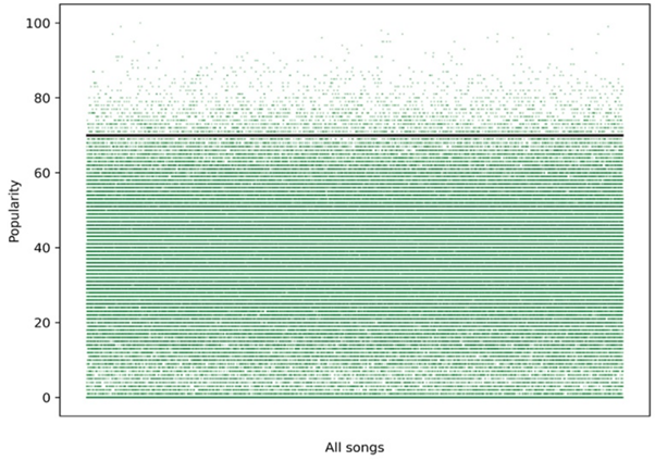 Figure 2. Scatter plot of popularity values with threshold in black
Balancing the dataset
Following this threshold selection, a new dataset was created to train our algorithm on balanced data with the same number of popular songs and unpopular songs. This under-sampling isn’t likely to result in a loss of important information as the balanced dataset still has a total of 7,670 rows.
 Figure 3. Unbalanced dataset (left) and balanced dataset (right)
Classification prediction with artist name
A logistic regression model was used to predict popularity with all the features of the binary unbalanced dataset in order to evaluate the importance of the features across the whole dataset.

With all the values, it was found that the artist_name variable is more than three times more important than any other attribute. However, as we are trying to predict the popularity of a song according to its audio features to help artists and labels succeed in the music industry, the artist_name variable isn’t really relevant. For example, Drake would not need this algorithm to assume his next song is going to be popular. Therefore, following this model prediction, artist_name was dropped from the x features.
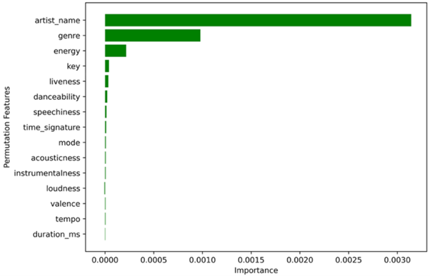 Figure 4. Feature Importance of Logistic Regression Model with artist_name
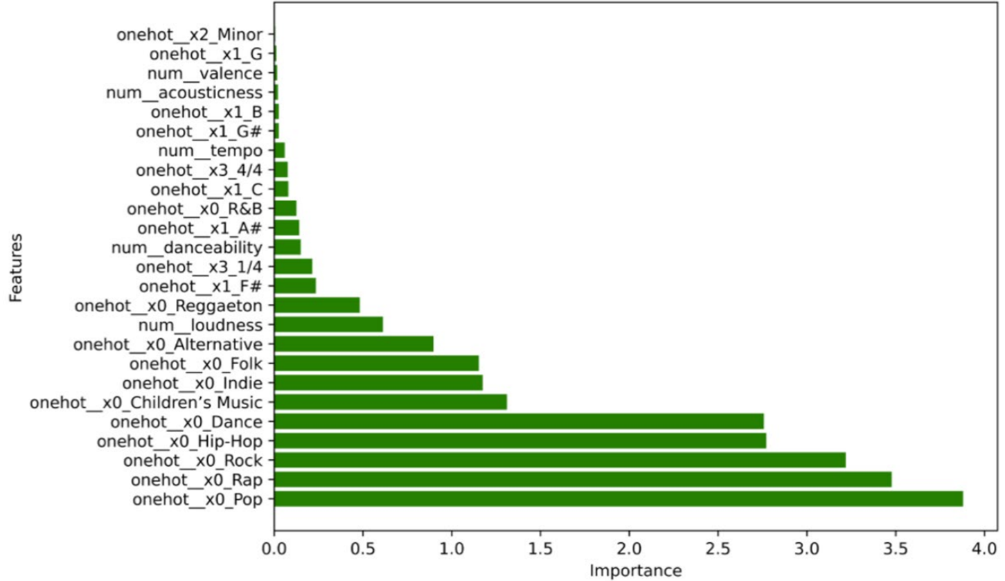 Figure 5. Feature Importance of Logistic Regression Model without artist_name
 Figure 6. Example tree for Random Forest Classifier with a max depth of 4 and one-hot encoded features


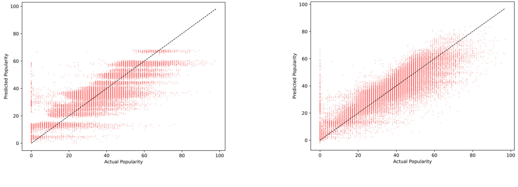 Figure 7. Predicted vs Actual Popularity without artist_name (left) and with artist_name (right)


